

1. Abstract
Foreign exchange is generated along with international trade, and its transaction is an important tool for international settlement of creditors’ rights and debts. Meanwhile, it has also become the most important financial commodity in this world. This paper mainly discusses the impact of multiple economic variables on the exchange rate prediction, including interest rate differential, inflation rate, and unemployment rate. And we choose the Canadian dollars and British pounds as our target currencies to see their exchange rates with the U.S. dollars. There are several machine learning models are selected to test the possibility of accurate prediction, such as LASSO regression, K-nearest neighbor regression, and supported vector regression. And the random forest model is considered the model with the best performance. Moreover, we also implement the training model on our trading strategy, which provides us a new vision regarding the future trend of exchange rate tracings.
2. Introduction
The exchange rate is one of the most important adjustment indicators in international trade. The fluctuations of exchange rate directly affect the cost and price of the commodity in the international market; therefore, it also directly affects the international competitiveness of the commodity as the cost of goods produced by a country is calculated in its own currency, to compete in the international market, the cost of its goods must be related to the exchange rate. Meanwhile, from the perspective of financial transactions, the exchange rate is also one of the important components of international finance. Whether in terms of liquidity or volume, the foreign exchange market is currently the largest financial market in worldwide. For investors and enterprises, it is particularly important to understand the mechanism of exchange rate fluctuations and establish exchange rate forecast models.
Therefore, in this project, we introduce and investigate several forecasting models, which include Linear Regression, Ridge Regression, Lasso Regression, Elastic Net Regression, Random Forest Model, and other machine learning models. In addition, we are also interested in the forecasting capability of Molodtsove and Papell’s Taylor rule model. By evaluating each model’s performance, we can select the most efficient models to construct our foreign exchange trading strategies. Here in this project, we mainly focus on the exchange rates between US Dollars to Canadian Dollars and US Dollars to British Pounds to further illustrate these models.
For the first part of this paper, we explain the fundamental concepts and basic frameworks. Moreover, we also discuss the economic variables that we are using in our models, and how are these variables correlated with foreign exchange rate fluctuations. And we are intended to explore as many independent economic variables as we can to construct the optimized exchange rate forecasting models.
The second part mainly focuses on illustrating the machine learning models and the Taylor rule model that we are using in this project. Their basic algorithms and evaluation criteria are discussed in this part as well. And we also report their prediction performance and determine the optimal forecasting model for each currency.
The following part demonstrates the trading strategies based on the selected machine learning models. And being able to accurately predict exchange rate trends can effectively help make proper trading, investment, or management decisions, such as hedging decisions, short-term investment decisions, and fixed asset investment decisions, etc.
Finally, we provide a brief conclusion regarding our work and theories. The models in this project are only based on basic economics theories and simplified real-world data. In addition, we expect more future steps as well to help us enhance the forecasting capabilities of our models, such as introducing more independent economics variables, analyzing investors’ confidence, and increasing the number of training data.
3. Conceptual Framework
3.1 Dependent Variable: Foreign Exchange Rates
The target currencies that we discuss in this project are British pounds (GBP) and Canadian Dollars (CAD). According to the statistics from International Monetary Fund (IMF), the British Pound has taken 4th place as the foreign exchange reserve as of 2021, and the Canadian dollar is listed as 6th place after the Chinese Renminbi. Due to geographical proximity to the United States and large volumes of international trading, the Canadian dollar is significantly affected by the neighboring country’s economy; meanwhile, as the United Kingdom and the United States share a close historical association and bilateral contemporary economics relationship, the British Pounds exchange rate have a strong connection with the United States economy as well. With the growing economies and stable currency prices, the two currencies are chosen to be measured relative to the US Dollar, which sets the US Dollars as the quote currency.
The foreign exchange rate is defined as the number of US Dollars that are able to exchange for one unit of foreign currency. Here in this project, the two exchange rates are written as followings:
An increase in either exchange rate (E) represents the appreciation of the foreign currencies, which are GBP and CAD in our project, or the depreciation of the quote currency USD. Thus, it also holds the same rule when there is a decrease in either exchange rates (E), it represents the depreciation of foreign currencies or the appreciation of quote currency.
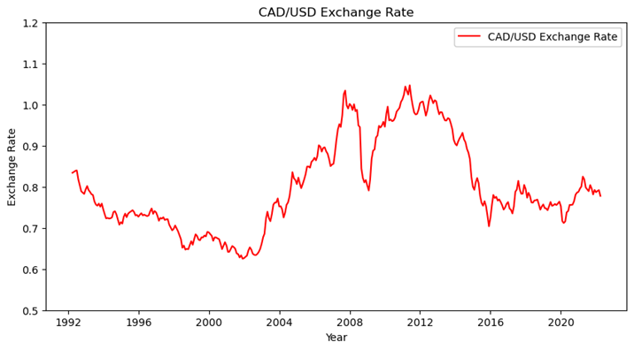
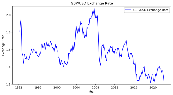
We collect the exchange rate data from the Federal Reserve Bank of St. Louis’s database and obtain the statistics starting from April 1st, 1992 to April 1st, 2022. The data are recorded on a monthly basis which we can conduct further investigation on their trend and pattern. Below are the graphs of the exchange rate of GBP and CAD:
3.2 Independent Variables
We obtain the independent economic variables from multiple resources, including FRED, the United States Census Bureau, and Organisation for Economic Co-operation and Development (OCED). And all the data are collected on a monthly basis as well. We believe the economic variables listed below should be considered as possible and relative indicators to the target variable, rather than the determinant and absolute terms.
3.2.1 Interest Rate Differentials (in,t)
By far the most visible and obvious power of many modern central banks is to influence market interest rates, which is one of the main tools that most central banks use to ease high inflation. An increase in the interest rate paid on deposits denominated in a particular currency will increase their rate of return, and this eventually leads to an appreciation of the currency since more investors are attracted to this type of deposit with a higher return and this specific currency has higher demand in the international market. Thus, the price of this particular currency is driven up, and we believe that the interest rates and exchange rates are positively related to each other.
Higher interest rates on dollar-denominated assets cause the dollar to appreciate, and higher interest rates on CAD or GBP-denominated assets cause the dollar to depreciate. In this case, the interest rate differential can be one of the momentous economic indicators for us to construct the exchange rate forecasting model.
3.2.2 Inflation Rate Differentials (𝝅)
People are willing to buy foreign currency because it has purchasing power for goods and services abroad. On the other hand, the domestic currency has purchasing power for the goods and services in the home market as well. Therefore, the exchange rate of the two currencies depends on the ratio of the purchasing power of the two currencies in the two countries. When inflation occurs in both currencies, the nominal exchange rate will be equal to the original exchange rate multiplied by the inflation rate of the two countries. Expectations of higher domestic inflation cause the expected purchasing power of domestic currency to decrease relative to the expected purchasing power of the foreign currency, thereby making the domestic currency depreciate.
Here we obtain the Consumer Price Index (CPI) growth rate for the United States, the United Kingdom, and Canada to calculate their differentials. The inflation rate for each country is calculated as follows:

3.2.3 Unemployment Rate Differentials (u)
The unemployment rate can be used to evaluate the overall employment condition of the labor force market in a specific time period, and the unemployment rate is also regarded as a significant indicator reflecting the entire economic status. A decrease in the unemployment rate shows that the overall economy is in a state of healthy development, which is conducive to facilitating market confidence and attracting foreign investment, and eventually promotes the appreciation of the currency. Conversely, a rising unemployment rate represents a slowdown or recession in the economy, which also implies a possibility of currency depreciation. Therefore, we use the two countries’ unemployment rate differential to understand the different job market conditions and expect that the unemployment rate differential has a negative relationship with the exchange rate.
3.2.4 Trading Balance (T)
With the fast development of international economic cooperation, the impact of trade on the various countries’ economies is also gradually expanding. Thus, in this project, we may also want to include bilateral trading balance as an independent economic variable, which is calculated as the difference between exports and imports. As the international trade balance release a market signal, it can help investors and traders to analyze the potential trend of one specific exchange rate: to increase exports, the country’s currency should be bought in order to buy its goods. As exports increase leads to decreases in deficit, therefore, a decline in deficit can be a signal of appreciation for the country’s currency. In our project, we assume it is negatively correlated with the exchange rate.
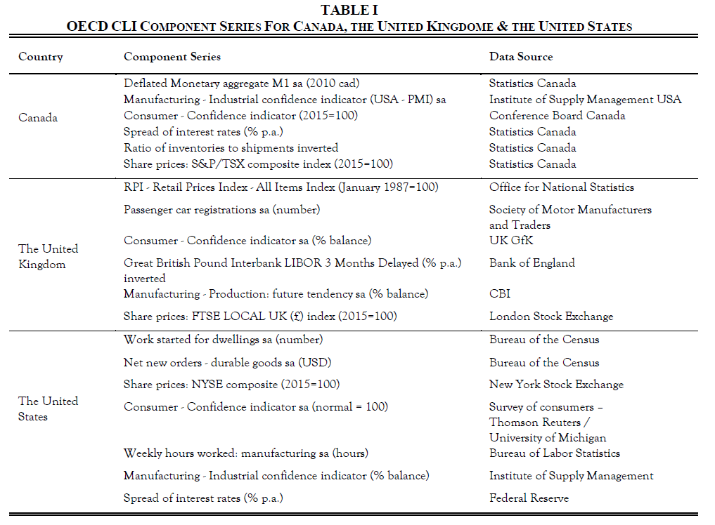
3.2.5 OCED Composite Leading Indicator (CLI) Differential
According to the OCED, the composite leading indicator (CLI) is designed to provide early signals of turning points in business cycles showing fluctuation of the economic activity around its long-term potential level. Moreover, the OCED CLI system is based on the growth cycle calculating approach, which includes business cycles and turning points in deviation-from-trend series. The component series for each country are selected based on various criteria such as economic significance and cyclical behavior.
The reasons why we prefer CLI rather than GDP data are as followings: first, CLI data publish more frequently than GDP as it updates monthly rather than quarterly like GDP does. Second, as OCED explains, the CLI is able to reflect more cyclical changes and economic turning points. Additionally, the Gross Domestic Product (GDP) is used as the reference for the identification of turning points in the growth cycle for all countries in the calculation of CLI. Hence, in this project, we use the two countries’ CLI differentials as an independent economic variable to predict the trend of the exchange rate.
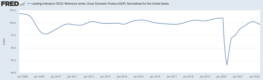
We can classify the economic cycle by looking at the amplitude-adjusted CLI, and we have four economic periods: (1) Expansion period, where CLI rises and its value is greater than 100; (2) Contraction period: CLI drops and its value is greater than 100; (3) Recession period: CLI declines and its value is less than 100; (4) Trough period: CLI rises and its value is less than 100.
The graph below shows that the United States experienced a recession period in 2008 as the CLI dropped from over 100 to nearly 97.5. Due to the COVID-19 pandemic, the same situation also happened in 2020 where the CLI dropped severely and reached the lowest point of 91.57 for the past 15 years. While starting in June 2020, the economy started to recover and entered into a trough period where CLI continued to grow mostly under 100 points until December 2021. The GDP CLI once again shows the tendency to decline and dropped below the 100-point standard, it is possible to enter a contraction period or even a new recession period since the new virus variant Omicron and high inflation are starting to affect the overall economy.
3.3 Model
A regression method is a supervised learning algorithm for predicting and modeling numerical continuous random variables. Annotated datasets with numerical target variables are one of the most important characteristics of regression tasks. That is, each observation has a numerical ground truth value to supervise the algorithm. Our use of machine learning for exchange rate prediction is a typical regression type of supervised learning algorithm. There is a total of 8 machine learning models used in this project, which include Linear Regression, Ridge Regression, Lasso Regression, Elastic Net Regression, K-Nearest Neighbor Regression (K-NN), Decision Tree Model, Support Vector Machine Model, and Random Forest Model, and we will explain each model accordingly in this section. For the models listed below, we used ten-fold cross-validations to tune the hyperparameters.
3.3.1 Linear Regression
Among all the machine learning models, linear regression is relatively more straightforward to understand, and it is one of the most commonly used algorithms for processing regression tasks. Linear regression fits a linear model with coefficients to minimize the residual sum of squares between the observed and linearly predicted values in the data. In this project, we use all the independent economic variables mentioned previously and construct a linear regression model. The equation for CAD is written as follows, and the equation for GBP also shares the same formula as below:
There are many drawbacks to linear regression as well. For instance, it generally performs poorly when the variables are nonlinear. And linear regression is not flexible enough to capture more complex patterns. It is also more difficult and time-consuming when we try to add the correct interaction terms or use polynomials. Therefore, in real practice, a simple linear regression is often replaced by regression methods that use regularization, such as LASSO regression, Ridge regression, and Elastic-Net regression. And we also introduce these regression methods to our project in the following sections.
3.3.2 Ridge Regression
The linear regression algorithm we discuss above uses the least squares method to optimize every coefficient. In the case of multicollinearity, the least squares method (OLS) is fair to each variable, but the variables may vary widely, which causes the observations to shift and move away from the true value.
Meanwhile, ridge regression analysis is a technique used for data with multicollinearity (independent variables are highly correlated). For ridge regression, it solves some problems of ordinary least squares by penalizing the coefficients (L2 regularization), that is, reducing the standard error by adding a degree of deviation to the regression estimate. The equation is as follows:

In the equation above, the first part calculates represents the difference between the observed value and our forecast value, which is the Sum of Squared Error (SSE). The L2 regularization element is the last portion, which is the penalty term for the square of the coefficient magnitude and penalizes features with higher slope values. In addition, lambda is the rate of shrinkage, if it is zero, then the model becomes linear regression. However, the larger lambda it is, our forecast becomes less sensitive to our predicting indicators, which leads to the model underfitting.
3.3.3 LASSO Regression
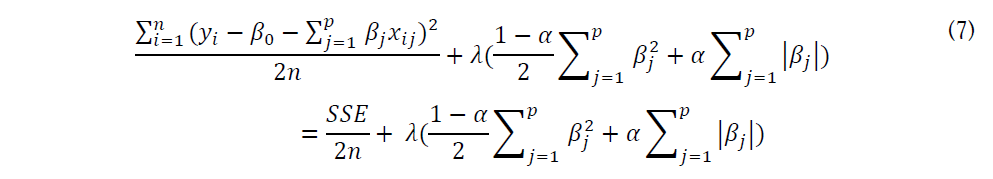
L1 regularization or LASSO regression adds the absolute value of the slope as a penalty term within the loss function. It helps us to clear out outliers by removing all data points with slope values less than a specific threshold, which in turn reduces variability and improves the accuracy of linear regression models. In this case, LASSO regression is different from Ridge regression as it uses the absolute value as the penalty function, rather than the squared value. Here shows how it is written:

As we can observe from the equation above, similar to the ridge regression, the first part calculates represents the difference between the observed value and our forecast value, which is the Sum of Squared Error (SSE). The L1 regularization element is the last part. In addition, lambda is the rate of shrinkage, we obtain the OLS when lambda equals 0. Meanwhile, the larger lambda it is, there are more coefficients are set to zero, and bias increases accordingly. If lambda decreases, then the variance is going to increase as well.
3.3.4 Elastic Net Regression
Elastic Net combines Lasso and Ridge regression into a single model with two penalty factors, which assigns the weights to the L1 norm and the L2 norm. By using this approach, the elastic net model is as sparse as pure Lasso regression, but at the same time, it also contains the same regularization power as ridge regression provides. Here shows how it is written:
As we can observe from the equation above, unlike ridge regression and ridge regression, it contains two different parameters to set, which are alpha and lambda. Here lambda still is the rate of shrinkage, we obtain the OLS when lambda equals 0. However, in terms of alpha, it is the weights for ridge regression and lasso regression. Thus, we need to find out the best combination of alpha and lambda to construct the optimal forecasting model, which can be done by using cross-validation. In this project, we are going to use 10-fold cross-validation to select the parameters.
3.3.5 K-Nearest Neighbors (K-NN)
K-Nearest Neighbors (K-NN) can solve both classification and regression problems. The K-nearest neighbor algorithm is “instance-based”, which means that it needs to retain the value of each training sample observation, and then predict the new value by searching for the most similar training sample. For the classification problem shown below, the testing unit, green dot, should be classified either into blue squares or red triangles. Here we assume the solid line circle is 3 distance units from the green dot, and the dashed line circle is 5 distance units away. If k = 3, then it is assigned to the red triangles because there are 2 triangles and only 1 square inside the solid line circle. However, if k = 5, the green dot is assigned to the blue squares as there are 3 squares vs. 2 triangles inside the dashed line circle.

When it comes to using K-NN to solve regression problems, the data labels are continuous variables rather than discrete variables. And the problem we face is no longer judging which class a sample belongs to like the above classification problem does. Here the regression problem can be solved by using the KNeighborsRegressor function. And the first step is the same as the classification algorithm, we need to find the K points closest to the point to be predicted. The second step we need to do is to take the average value of these K points as the predicted value of the forecasting point. Thus, we are able to use K-NN in this project to forecast future exchange rates.
3.3.6 Classification And Regression Tree (CART)
According to the different types of data processed, decision trees are divided into two categories: classification decision trees and regression decision trees. Classification decision trees can be used to deal with discrete data, and regression decision trees can be used to deal with continuous data. For a standard decision tree, it usually consists of nodes and directed edges. And there are two types of nodes: internal nodes and leaf nodes. Internal nodes represent a feature or attribute (ellipse box in the graph below), and leaf nodes represent a category or a value (square box in the graph below). When the dependent variable of the dataset is a continuous value, the regression tree can be used for fitting and forecasting, and the mean value of the leaf node is used as the predicted value of the node.
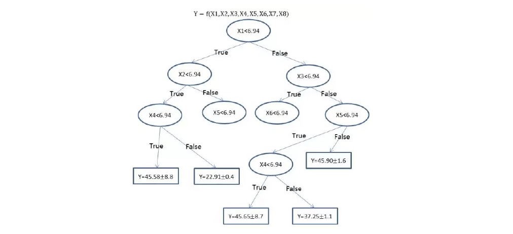
When using a decision tree for classification or regression tasks, we start from the root node to test a certain feature of the sample, and then assign the sample to its child nodes according to the test results; at this time, each child node corresponds to a value of the feature. Samples are tested and assigned recursively in this way until a leaf node is reached. Regression trees may have some drawbacks, for example, regression tree can be unconstrained, which means that a single tree can easily lead to overfitting results. However, decision trees can also learn nonlinear relationships and they are robust to outliers. Thus, we use this algorithm to generate predictions in this project as well.
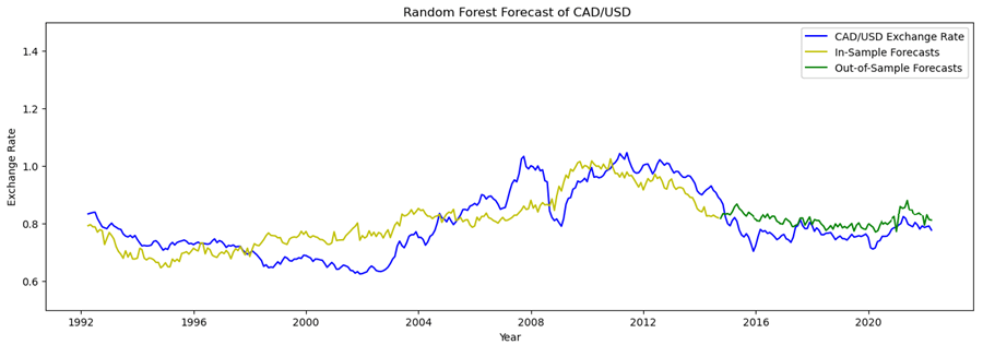
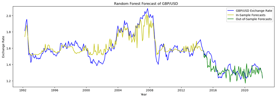
3.3.7 Random Forest
Random Forest Regression is an important application branch of the Random Forest algorithm. In the training phase, the random forest regression model uses bootstrap to randomly extract samples and features, establishes multiple unrelated decision trees, and obtains prediction results in parallel; then in the prediction phase, each decision tree can generate a prediction result by extracting samples and features, and then the algorithm retrieves regression prediction result of the entire forest by synthesizing the results of all trees and taking the average. This process is called bagging.
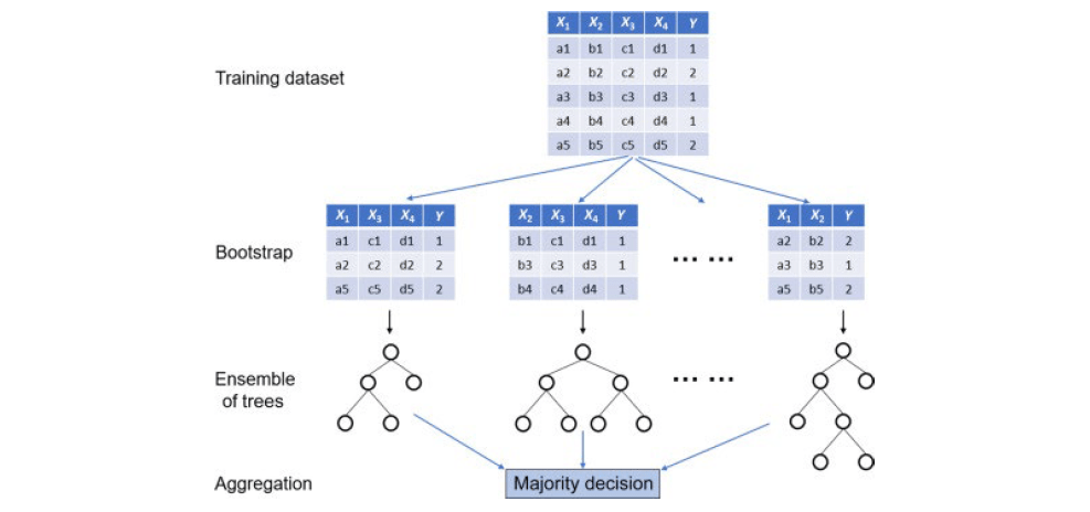
In the field of machine learning, the random forest regression algorithm is more suitable for regression problems compared with other algorithms and models. Generally, it is one of the most efficient models in situations where there is a nonlinear or complex relationship between features and labels. And it is insensitive to noise in the training set, which is more conducive to obtaining a robust model. Moreover, the random forest algorithm is more robust than a single decision tree as it assembles a set of unrelated decision trees. But the random forest algorithm also has its own shortcomings. For example, its main disadvantage is complexity. Since we need to connect a large number of decision trees together, they require more computational resources. Also due to their complexity, they require more time in the training phase compared with other similar algorithms. The random forest regression algorithm is used in scenarios with relatively low data dimensions and high accuracy requirements. Thus, we include random forest regression algorithms in this project.
3.3.8 Support Vector Regression (SVR)
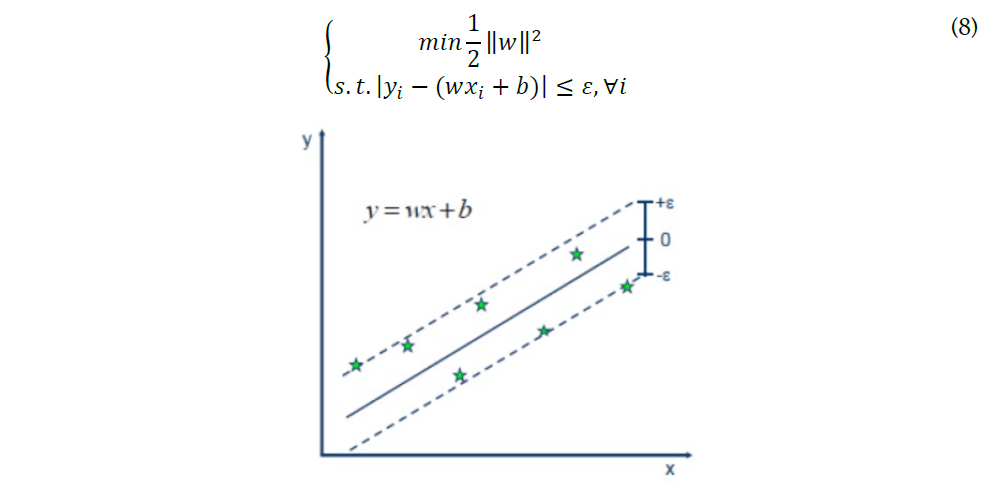
Support Vector Regression (SVR) is an important application branch of Support Vector Machine (SVM). SVR is a regression model, which is mainly used to fit numerical values and is generally used in scenarios with sparse features and a small number of features. Through the SVR algorithm, a regression plane can be found and all the data in a set have the shortest distance from this plane.
SVR creates an “interval band” on both sides of the linear function with the margin ϵ (also called a margin of tolerance, which is an empirical value set manually), and no loss is calculated for all samples that fall within the margin band, which means that only the support vector will affect its model. Then we can achieve the optimized model by minimizing the total loss and maximizing the margin. The demonstration chart and constrain equations are shown below:
4. Results Evaluation
To estimate the performance of each machine learning model in this project, we choose Mean Square Error (MSE) as our evaluation metric. For a regression model to be considered a good model, the MSE should be as small as possible. Here is the formula for MSE:

The performance for each model is listed below:
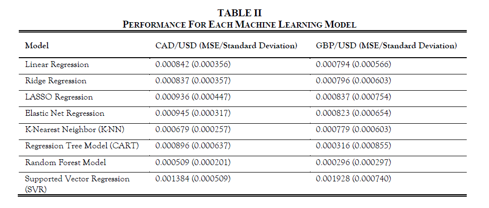
The statistics above show that the random forest model achieves the lowest MSE, which indicates that it performs better than other models. Thus, we expect that we should choose the random forest model as our forecasting model with the selected variables we mentioned previously. Below is the graph showing the coefficient for each independent variable.
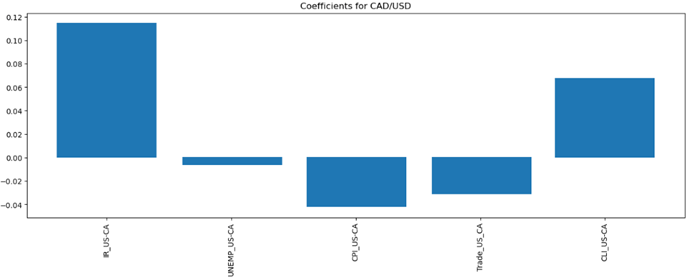
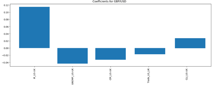
The graphs generally follow our expectations. Interest rate differential and CLI GDP are positively correlated with the exchange rate; While the unemployment rate, inflation rate, and trade deficit are negatively correlated with the target variable.
5. Taylor Rule
5.1 Methodology and Model
The Taylor rule is one of the most commonly used fundamental monetary policy rules, which was proposed by Stanford economist John Taylor based on the actual economic data of the United States. The Taylor rule describes how short-term interest rates adjust to the changes in inflation and output. Although it only contains a basic form, it has a profound impact on the later study of monetary policy rules. If the central bank adopts the Taylor rule, the choice of monetary policy constructs a pre-commitment mechanism, which is able to solve the problem of time inconsistency in monetary policy decision-making. The formula is listed as follows:

This rule assumes the equilibrium federal funds rate of 2% above inflation, which is the sum of the inflation rate (π) and the “2” on the right side of this equation. And the inflation gap, (π-2), infers that the federal funds rate (i_ff) fluctuates with half the difference between actual and targeted inflation. And the (y_t-y ̅) represents the percent deviation between the current real GDP and the long-term linear trend in GDP.
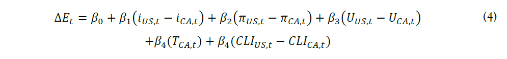
In terms of using the Taylor rule as a forecasting tool, Molodtsove and Papell proposed a forecasting model for the log nominal exchange rate using the inflation rates (π_t^us) and GDP gaps (φ_t^us) in two countries, which is called the “homogenous, symmetric Taylor rule model without smoothing” in their paper (Molodtsove & Papell, 2009). Their model is shown below:

Following their methodology, we use monthly CPI data, countries’ GDP, interest rate, and exchange rates of the United States, Canada, and the United Kingdom from Jan-1997 to Jan-2022 to examine the out-of-sample exchange rate predictability with Taylor rule fundamentals. In addition, Molodtsove and Papell calculate the output based on linear time trend, quadratic time trend, and Hodrick and Prescott’s (HP) (1997) trend. Thus, we evaluate the output of each one accordingly.
5.2 Statistics Testing and Evaluation
To test whether the forecasts are better than a random walk model, we conduct three statistical tests, which are Diebold-Mariano-West (DMW), Clark-West (CW), and the basic MSE evaluation we implemented previously.
5.2.1 Diebold-Mariano-West (DMW) Test
The Diebold-Mariano-West test is based on two papers: Diebold and Mariano (1995) and West (1996). The hypothesizes and DMW test formulas are listed as follows:
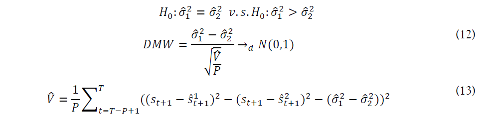
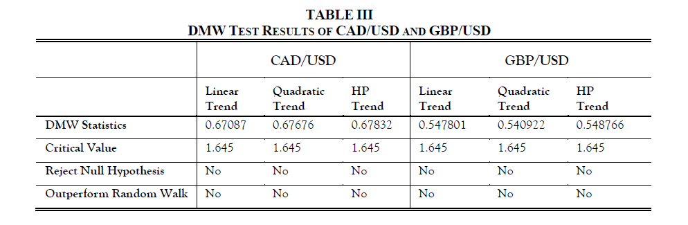
According to the theory of the DMW test, H0 will be rejected at level α if DMW > z, where z is the standard normal. Thus, the three methods used in Taylor Rule out-of-sample forecasts don’t beat the random walk based on the results below.
5.2.2 Clark-West (CW) Test
The Clark-West Test based on Clark and West (2006) is a refinement of the DMW test. It indicates the DMW test under-rejects the null hypothesis. The equation and test results are listed as follows:
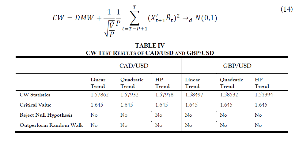
According to the CW test results shown above, we may conclude that the three methods used in Taylor Rule out-of-sample forecasts don’t beat the random walk.
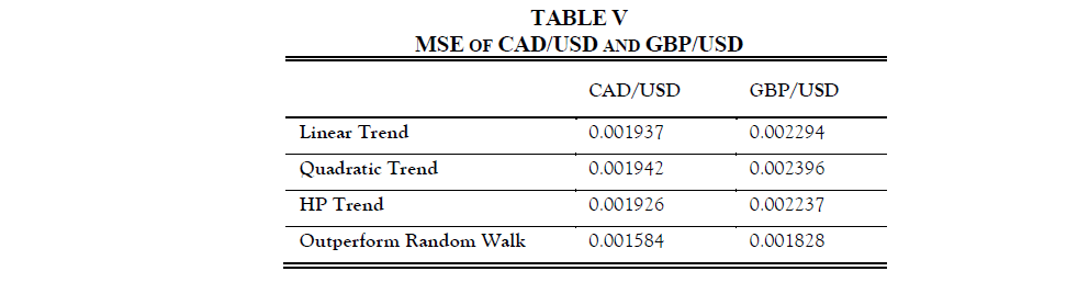
5.2.3 Mean Squared Error (MSE)
By using the same approach that we used previously for machine learning models, we calculate the mean squared error of the Taylor rule model’s forecasting results. However, the Taylor rule model still does not outperform the random walk for both CAD and GBP exchange rate forecasts. Statistics are listed as follows:
6. Trading Strategy and Additional Comment
The U.S. dollar index has entered a new increasing cycle. The Federal Reserve has raised interest rates several times during the pandemic in an effort to reduce the inflation rate and unemployment rate. Thus, the U.S. dollar has broken through the consolidation period and entered a new rising stage. Since the beginning of 2022, the Federal Reserve has responded to the high inflation and high unemployment caused by the epidemic through the monetary policy of raising interest rates. And from 2021 to the present, the tightening monetary policy has led to the appreciation of the US dollar relative to either low-yielding currencies (Euro, Japanese yen, Swiss franc) or high-yielding currencies (Australian dollar, New Zealand dollar, Norwegian krone); investors bought a large number of US dollar assets, which led to the rise of the US dollar and pushed up the US dollar index.
The US dollar is likely to continue to perform strongly against the Canadian dollar. Also, USD/CAD is likely to continue its bullish trend for the future periods in 2022 as the Bank of Canada announces that it is likely to slow down rate hikes in the coming months. At the same time, based on our model analysis, the United States still maintains a relatively stronger exchange rate trend as it has a higher interest rate.
The main economic exchanges between the United Kingdom and the United States have a strong correlation, and the trend of GBP/USD is almost the same as that of EUR/USD in a falling channel. The Fed may still raise interest rates in the future. Just as our analysis is consistent, the GBP/USD exchange rate will continue to decline in the short term. In the medium and long term, the monetary policies of European countries and the recovery of the overall European economy due to the impact of the epidemic are difficult to predict in the future, and there are still uncertainties.
7. Conclusion
This paper investigates the impact of interest rate, inflation rate, unemployment rate, international trade balance, and CLI index on the exchange rate prediction. And we have chosen the Canadian dollars and British pounds as our target currencies to see their exchange rates with the U.S. dollars. We believe that all the independent variables’ correlation with the target variable meets our initial expectations. There are various machine learning models are selected to test the possibility of accurate prediction, and the random forest is considered the model with the best performance among them according to the MSE evaluation. Moreover, we also use the Taylor rule forecasting model proposed by Molodtsove and Papell to investigate its forecasting capability. In the end, we decide to use the random forest model and implement it in our trading strategy, which we believe that the U.S. dollar will maintain its strength against other currencies given its rate hike situation.
8. Future Work
According to the graph and statistics shown above, we believe that the overall results are promising, but there are still many places that we can adjust to improve the performance.
8.1 More Independent Variables
Having more independent variables can be beneficial for our testing accuracy. More variables mean that there are more perspectives for us to enhance the predicting capabilities of our models. The current models and independent variables are simplified for a more straightforward understanding. Our potential independent variables for this research can be investor’s confidence, producer price index, personal income, and household consumption expenditure.
8.2 Different Machine Learning Models
The models we have introduced so far are just some common models and fundamental theories in the field of machine learning. More advanced algorithms can help us better understand the laws of exchange rate fluctuations and their possible future trends. In the future, we can introduce more different models, such as long short-term memory networks, multilayer perceptron, and deep belief networks.
8.3 Large Training Data Samples
The foreign exchange market is a market without time and space barriers as it maintains 24-hour consecutive trading across the world. It is the largest financial market with the greatest daily trading volume as well. Thus, the price of foreign exchange fluctuates continuously every day or even every second. The reason why we select foreign exchange prices on a monthly basis is to match as many independent variables as possible, and many economic data are not available for a daily basis record. Therefore, we hope to expand our data sources and have a larger training data sample, so that we can receive more precise results regarding the laws of foreign exchange changes.
Special Thanks
This paper is completed under the instruction of Professor Randall Rojas. I would like to express my thanks to him as he gave me a lot of valuable advice on the research topic. Meanwhile, I also appreciated the suggestions given by my friend Xu Haixiang, who gave me some machine learning theory explanations. In the end, my partner Quan Shengjie provided many inspiring points, which significantly helped me train my machine learning models. Without the support of the people mentioned above, it would become a really tough goal for me to accomplish this capstone paper.
References
- Board of Governors of the Federal Reserve System (US), Federal Funds Effective Rate [FEDFUNDS], retrieved from FRED, Federal Reserve Bank of St. Louis; https://fred.stlouisfed.org/series/FEDFUNDS, November 14, 2022.
- Organization for Economic Co-operation and Development, Interest Rates: Immediate Rates (< 24 Hrs): Call Money/Interbank Rate: Total for Canada [IRSTCI01CAM156N], retrieved from FRED, Federal Reserve Bank of St. Louis; https://fred.stlouisfed.org/series/IRSTCI01CAM156N, November 14, 2022.
- Organization for Economic Co-operation and Development, Consumer Price Index: All Items for the United States [USACPIALLMINMEI], retrieved from FRED, Federal Reserve Bank of St. Louis; https://fred.stlouisfed.org/series/USACPIALLMINMEI, November 14, 2022.
- Organization for Economic Co-operation and Development, Consumer Price Index: All Items: Total: Total for Canada [CANCPIALLMINMEI], retrieved from FRED, Federal Reserve Bank of St. Louis; https://fred.stlouisfed.org/series/CANCPIALLMINMEI, November 15, 2022.
- U.S. Census Bureau (2022). Trade in Goods with Canada, 1992-2022. Retrieved from https://www.census.gov/foreign-trade/balance/c1220.html#, November 15, 2022.
- U.S. Census Bureau (2022). Trade in Goods with United Kingdom, 1992-2022. Retrieved from https://www.census.gov/foreign-trade/balance/c4120.html, November 15, 2022.
- OECD (2022), Unemployment rate (indicator). doi: 10.1787/52570002-en (Accessed on 15 November 2022)
- Organization for Economic Co-operation and Development, Immediate Rates: Less than 24 Hours: Call Money/Interbank Rate for the United Kingdom [IRSTCI01GBM156N], retrieved from FRED, Federal Reserve Bank of St. Louis; https://fred.stlouisfed.org/series/IRSTCI01GBM156N, November 14, 2022.
- Organization for Economic Co-operation and Development, Consumer Price Index: All items: Total: Total for the United Kingdom [GBRCPALTT01IXNBM], retrieved from FRED, Federal Reserve Bank of St. Louis; https://fred.stlouisfed.org/series/GBRCPALTT01IXNBM, November 15, 2022.
- Board of Governors of the Federal Reserve System (US), U.S. Dollars to U.K. Pound Sterling Spot Exchange Rate [EXUSUK], retrieved from FRED, Federal Reserve Bank of St. Louis; https://fred.stlouisfed.org/series/EXUSUK, November 14, 2022.
- Organization for Economic Co-operation and Development, Leading Indicators OECD: Reference series: Gross Domestic Product (GDP): Normalised for the United States [USALORSGPNOSTSAM], retrieved from FRED, Federal Reserve Bank of St. Louis; https://fred.stlouisfed.org/series/USALORSGPNOSTSAM, November 14, 2022.
- Organization for Economic Co-operation and Development, Leading Indicators OECD: Reference series: Gross Domestic Product (GDP): Normalised for Canada [CANLORSGPNOSTSAM], retrieved from FRED, Federal Reserve Bank of St. Louis; https://fred.stlouisfed.org/series/CANLORSGPNOSTSAM, November 14, 2022.
- Organization for Economic Co-operation and Development, Leading Indicators OECD: Reference series: Gross Domestic Product (GDP): Normalised for the United Kingdom [GBRLORSGPNOSTSAM], retrieved from FRED, Federal Reserve Bank of St. Louis; https://fred.stlouisfed.org/series/GBRLORSGPNOSTSAM, November 14, 2022.
- IMF. 2017. World Currency Composition of Official Foreign Exchange Reserves; https://data.imf.org/regular.aspx?key=41175 November 14, 2022.
- Heipertz, J., Mihov, I., & Santacreu, A. M. (2017). Managing Macroeconomic Fluctuations with Flexible Exchange Rate Targeting. https://doi.org/10.20955/wp.2017.028
- OECD . (n.d.). OECD Composite Leading Indicators: Turning Points of Reference Series and Component Series. OCED. https://www.oecd.org/sdd/leading-indicators/CLI-components-and-turning-points.pdf
- Molodtsova, T., & Papell, D. (2009), Out-of-sample exchange rate predictability with Taylor rule fundamentals. Journal of International Economics, 77(2), 167-180.
- Pfahler, F. J., (2021). Exchange Rate Forecasting with Advanced Machine Learning Methods. MDPI. https://www.mdpi.com/1911-8074/15/1/2/html
- Pathirana, V. K. (2015), Nearest Neighbor Foreign Exchange Rate Forecasting with Mahalanobis Distance. https://core.ac.uk/download/pdf/154471192.pdf
- Pfahler, F. J., (2021). Exchange Rate Forecasting with Advanced Machine Learning Methods. MDPI. https://www.mdpi.com/1911-8074/15/1/2/html

留下评论